


The train stays at the factory.
With ONIS 20kV.
For a rail manufacturer, we measured train input impedance directly at the production site. With ONIS 20kV, our independently developed medium-voltage solution, measurement became part of the on-site validation process.
ONIS 20kV: developed by morEnergy, deployed at the customer’s site
The challenge and our solution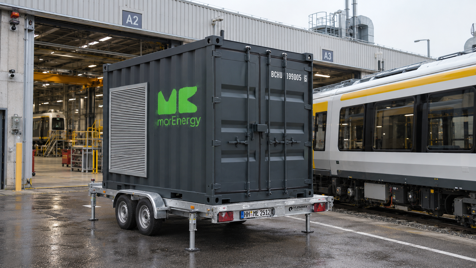
The measurement equipment comes to the train.
Delivery
Bring ONIS 20kV to the production site.
Train measurement
Measure the train where it is built.
The container travels. The train stays at the factory.Less transport, personnel and coordination effort reduces the associated costs.
Durations from this deployment: delivery on the project’s route and measurement of one train. Preparation, test-environment measurements and evaluation are not fully included. Duration depends on location and test scope.
The measurements were needed.
Getting there took effort.
Determine frequency-dependent train input impedance. In different operating states. Directly at the production site.
One train. Many journeys.
Previously, measurements required an external test facility. Scheduling, transporting the train and returning it involved several weeks of lead time.
The factory lacked the specialist equipment and experience for on-site measurement.
The measurement equipment comes to the train.
With ONIS 20kV, we scaled our ONIS technology to medium voltage and integrated it into a mobile 10-foot container.
Why this measurement matters.
The train and its supply interact electrically. Resonances can amplify voltage and current components; the operating configuration can also change the input characteristics. Our on-site measurements provide a dataset for assessing relevant frequency regions and interpreting differences between configurations.
The examples use synthetic models, not customer measurement data. They do not show a finding on the customer’s train and are not proof of stability.
Understanding resonancesInteractive RLC equivalent model · Not a train measurement
The current stays the same.
In the simplified parallel RLC equivalent circuit, the current excitation is held constant.
The resonance changes.
The weaker the damping, the higher the impedance at resonance.
The response becomes larger.
For the same current excitation, the higher impedance produces a larger voltage response.
What happens when damping is low?
Reduce the damping. The excitation stays the same while the resonance peak grows.
How strongly does the circuit respond to continuous sinusoidal excitation?
See the higher-frequency component on the sine wave.
A higher-frequency current component continuously excites the circuit at resonance. The resulting voltage is superimposed on the fundamental sine wave. Reduce the damping: the ripple on the sine wave grows while the excitation stays the same.
Illustrative equivalent model. Not a train measurement or acceptance limits. Axes normalized.
The model behind the plots
Illustrative equivalent model, not a train measurement. The axes are normalized. The frequency response shows sinusoidal current excitation. The time waveform shows steady state: a prescribed fundamental with a continuous superimposed voltage component at resonance. Both views use the same RLC circuit and damping value; neither represents actual train values or acceptance limits.
For the ideal parallel RLC circuit, f₀ = 1 / (2π√(LC)). For the same current excitation, normalized voltage response is proportional to |Z_RLC| / Z₀. The reference uses d = 0.8. This model does not describe a specific train or supply topology.
The time waveform is the sum of the fundamental and a higher-frequency voltage component:
Û₁ is the fundamental voltage amplitude. The amplitude Ûh of the superimposed voltage component follows from the fixed current excitation and the equivalent-circuit impedance:
Îh stays constant as the slider moves. In this example its frequency is at resonance: fh = f₀ = 12f₁. The equivalent-circuit impedance is real there, so this voltage component is shown without an additional phase shift. Less damping increases the impedance at this frequency and therefore increases Ûh. The fundamental, frequency ratio and current amplitude are illustrative choices. The plotted total voltage is normalized by Û₁.
What this means for engineering evaluation
Our deployment focused on characterizing the frequency response at the train input and assessing resonances. The train and its supply form an electrical system: converters, filters and controls interact with the network. Unfavorable interactions can amplify voltage and current components and place additional stress on equipment.
A simplified parallel RLC equivalent circuit illustrates the principle. Its impedance rises near resonance. For the same current excitation, weaker damping produces a larger voltage response:
Here, ZRLC is the impedance of the simplified RLC equivalent circuit. ΔU and ΔI are the complex voltage and current components at the frequency being considered.
Back to the project: With ONIS 20kV, we made the train’s input characteristics measurable on site. This gave the validation engineers a dataset for assessing relevant frequency regions. The weak damping in the plot is an explanatory example, not a finding on the customer’s train.
Why compare operating states?Synthetic comparison of operating states · Not a customer finding
2 operating configurations
Measured separately. Differences interpreted in context. Phase and the real part of admittance were considered alongside magnitude.
An abnormal response calls for investigation.
A negative real part alone does not prove system instability. Interaction with the supply and measurement conditions belong in the assessment.
A feature revealed by comparing operating states.
Enable the illustrative state with an abnormal response. In the highlighted frequency band, the real part becomes negative and phase exceeds +90°.
Synthetic example, not a customer finding. Neither a standards test nor proof of stability.
Notes on the synthetic example
Hypothetical fault scenario, not a customer finding. Both curves come from an independent synthetic model. Frequency is dimensionless and admittance uses a common reference. This illustration is neither a standards test nor proof of stability.
A negative real part in a frequency band can indicate behavior that counteracts positive damping. This calls for a closer investigation of interaction with the supply. In the scalar model, it corresponds to a phase angle outside ±90°.
A negative real part alone does not prove system instability. Likewise, an unremarkable frequency region does not guarantee stability for every operating and supply condition. Applicable criteria, measurement conditions and possible effects of existing harmonics belong in the engineering assessment.
In our deployment, this meant measuring the configurations separately and interpreting their differences. The abnormal behavior in the example illustrates why this approach is useful; it does not describe a fault encountered in the project.
The measurement task in detail
Input admittance
The measured quantity was input admittance — the reciprocal of input impedance.
Two configurations
The train’s input characteristics were measured in two operating configurations.
Evaluate together
The manufacturer’s validation engineers and morEnergy interpret the results in their engineering context.
To validate new train series, our customer needed to determine frequency-dependent input impedance in different operating states. Previously, this required measurements at an external test facility. Scheduling, transporting the train and returning it involved several weeks of lead time and logistical coordination.
The factory lacked the specialist equipment and experience to carry out these measurements locally. This was the starting point for the collaboration with morEnergy.
Measure train input impedance directly at the production site using a transportable medium-voltage solution.
The ONIS 20kV container solution was developed by morEnergy. We scaled our ONIS technology to medium voltage and integrated it into a mobile 10-foot container. During the on-site deployment, we used it to measure the train’s input characteristics in different configurations.
The measured quantity was input admittance, the reciprocal of input impedance. Both describe the same relationship between voltage and current perturbations at the train’s electrical input:
Here, s denotes the operating state. The following interactive examples explain why frequency response and multiple operating states matter. They illustrate the questions behind our deployment; the curves are generated independently of the customer project.
Measurements gain meaning.
Through their context.
A sound assessment required more than recording the train’s response curves.
Measure the test environment too.
We first measured the test environment without the train connected. This allowed us to consider the influence of the test track and its connection infrastructure during evaluation. The train was measured in two operating configurations.
Interpret unusual phase points.
During evaluation, we examined unusual phase points alongside existing voltage harmonics. This helped us interpret harmonic-affected points rather than treating every excursion as instability.
Compare with references.
We compared the results with simulations and previous impedance measurements. Good agreement supported confidence in their use for engineering evaluation.
Simple measurement. Expert evaluation.
The app simplifies measurement execution for additional users. The manufacturer’s validation engineers and morEnergy specialists are available to support interpretation.
How the results can be used
The deployment demonstrated that the mobile solution could perform the measurement task at the production site. A sound assessment required more than recording the train’s response curves.
Engineers can use this information to decide whether further investigation or changes to configuration, controls or components are appropriate. This case study does not claim a specific component change in the project.
The train stays at the factory.
Measurement becomes part of the workflow.
ONIS 20kV is now part of the customer’s validation process.
Take the train to the measurement.
Several weeks of lead time for scheduling, transport and the return journey.
Planning lead timeBring measurement to the train.
One working day for delivery and one working day for train measurement in this deployment. The train stays at the production site.
Two individual work steps in this deploymentThese are different measures of time: planning lead time and individual work steps. Additional preparation, test-environment measurements and evaluation are not fully included in the two working days.
Train transport
No train transport to and from an external test facility for this measurement task.
Personnel effort
Less personnel effort through a simpler workflow and app-supported operation.
Coordination
Less coordination around train transport and external testing appointments.
Reducing these activities lowers the associated costs. The actual savings depend on transport distance, test scope and organization.
The benefit for the ongoing validation process
The durations describe delivery and train measurement. Additional preparation, test-environment measurements and evaluation depend on the task. The previous planning lead time and these two work steps are different measures of time.
ONIS 20kV is now part of the customer’s validation process. The transportable container can also be deployed at other locations. For new measurement tasks, the equipment comes to the train, removing the need to transport it to an external test facility for these measurements.
App-supported operation simplifies execution, reduces coordination and personnel effort, and makes measurement accessible to additional users. morEnergy specialists are available to support evaluation.
Complex electrical behavior?
Let’s discuss it.
Resonances, unexpected harmonics, or interactions with the supply? We combine on-site measurement, our ONIS technology, and engineering expertise to investigate your system and provide a sound basis for your next steps.