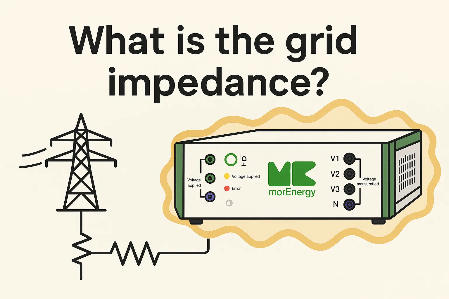
Grid impedance is a decisive factor for the behavior and stability of power grids. It describes the interaction between voltage and current and has a significant influence on how electrical energy flows through the grid. Precise knowledge of the grid impedance is essential, as deviations not only affect the quality of the power supply, but can also cause resonances in the grid. These resonances can lead to significant problems by amplifying unwanted oscillations and thus damaging the grid and connected devices. This article explains the basics of grid impedance and its effects on resonances and grid stability in more detail.
What is power quality and how is it measured?
The properties of an electrical power supply network are described using a large number of parameters. The calculation of these parameters, such as the grid frequency or the voltage distortion factor THD, is defined in various standards and guidelines. These also contain specifications and limit values that must be adhered to during operation in order to ensure a reliable and fault-free power supply.
For the use of electrical energy in AC grids, a constant grid frequency, a constant supply voltage and a perfect sine wave shape of the supply voltage are desirable. However, deviations occur in practice due to the spatial expansion and the large number of different consumers and generators. The consumption of electrical energy causes currents, which in turn lead to voltage drops across the lines and components of the grid. The level of the supply voltage for a grid user is therefore dependent on the interaction of all voltage drops in the grid area that supplies the user. Another example is the variation of the grid frequency. In order to maintain a constant grid frequency, there must be a perfect balance between generator output and consumer output at all times, i.e. the same amount of energy must be fed into the grid as is currently being demanded. An imbalance leads to a corresponding drop or rise in the grid frequency. There is therefore an interplay between the generation and consumption of electrical energy that influences the various parameters. In general, it can be said that every electrical consumer generates grid repercussions during operation as well as when it is switched on and off. The large number of connected consumers therefore influences the grid through interference emissions and non-linear current-voltage characteristics, as is increasingly the case with power electronic devices.
The term “power quality” refers to the correspondence between the required characteristics of the mains voltage and current and the characteristics of the electricity supplied. If the parameters are within the limits defined in the applicable standards and directives, connected devices can be operated correctly and it can be assumed that they will not be damaged.
The terms power quality and voltage quality are often used interchangeably, as voltage has a significant influence on power quality for grid users. However, the term power quality includes both voltage and current quality. The evaluation criteria for power quality include
- Mains frequency
- Slow voltage changes/voltage level
- Rapid voltage changes
- Flicker
- Voltage dips
- Short/long interruptions
- Transient
- Asymmetries
- Harmonics
The measurement of power quality is becoming increasingly important with the progressive integration of renewable energies and the increased use of power electronic devices. A distinction can be made between two types of power quality measurement: short-term grid analyses and long-term, permanent monitoring.
In short-term grid analyses, the power quality at a location is determined in order to record the current status of the grid. If, for example, a production plant is to be built at this location, the knowledge gained can be used to determine whether the location is suitable. Determining power quality can also help to develop suitable measures to improve power quality in the event of recurring problems or production plant failures. With permanent monitoring, the power quality in the grid is permanently monitored in order to detect long-term trends at an early stage and to take suitable countermeasures in good time should harmful changes occur.
What are harmonics?
The frequency components in the grid voltage or current that deviate from the nominal grid frequency (50 Hz in the European grid) are referred to as harmonics. If they correspond to an integer multiple of the fundamental frequency, i.e. 100Hz or 150Hz, they are also called harmonics. For example, 150Hz is the 3rd harmonic, as it is three times the fundamental frequency. The mains voltage that the mains user receives is made up of the superimposition of the fundamental frequency with all harmonic components. The harmonics are correspondingly undesirable frequencies that degrade the quality of the mains voltage, as this is ideally represented by a perfect sine wave.
Harmonics and harmonics are caused by non-linear equipment. This means that the current drawn from a non-linear load or fed in by such a generator is not sinusoidal or is switched on and off periodically. The currents cause corresponding voltage drops of different frequencies, which then distort the mains voltage. Non-linear loads include energy-saving lamps, inverters and switching power supplies.
Harmonics are bad for equipment and devices connected to the mains and can lead to malfunctions, overloading, ageing, loss of performance or damage and destruction. Harmonics are also a problem for cables, as they must be designed for the currents flowing through them. If you look at a symmetrically loaded three-phase network, for example, you can see that the fundamental vibrations in the neutral conductor cancel each other out due to superimposition, but the harmonics add up. This additional load must be taken into account when designing the cables.
Filters (suction circuits), for example, can be used to avoid and reduce harmonics. These filters have a very low impedance for the corresponding frequencies and then dissipate the corresponding components.
What is power quality monitoring?
Power quality monitoring is the continuous monitoring of the grid or a system with regard to power quality parameters. Continuous measurement allows trends and problems to be identified at an early stage so that measures can be developed in good time to prevent further damage and faults.
Even in the event of faults and unforeseen failures, the data recorded by continuous monitoring allows conclusions to be drawn about the cause. They can be used to develop remedial measures so that the problem does not occur again in the future and can be solved sustainably. Another useful application is the use of power quality data for grid planning. It can be used to identify where an existing grid still has free capacity or is already being used at maximum capacity. However, power quality monitoring can also help to save energy, as unwanted power flows in the grid can be detected.
What are impedances and what is the mains impedance?
The behavior of electrical components and circuits is fundamentally dependent on the frequency f of the operating voltage and current. Analogous to DC circuits, in which the ratio of voltage U and current I is characterized by the resistance value R, the impedance describes the ratio of voltage U and current I at any given frequency. The impedance therefore characterizes the frequency-dependent resistance of electrical components such as a coil, a capacitor or a resistor. It is therefore an important variable in complex alternating current technology and is identified by the formula symbol Z.
As a complex quantity, the impedance is made up of a real part R and an imaginary part X and can be represented as a pointer in the Gaussian number plane. The imaginary part X is also referred to as reactance. As an alternative to representation via the real and imaginary parts, the impedance can be characterized via the magnitude |Z| and the phase ϕ.

The reciprocal value of the impedance is often used, which is referred to as admittance Y and is related to the impedance as follows:
$$Y = \frac{1}{Z}$$
The impedance ZL of an ideal coil with inductance L increases linearly with frequency f and is purely imaginary. It is calculated using the following equation
$$Z_L = j 2 \pi f L$$
and is shown in Figure 1. An inductance of 1mH was selected for the plot.

In contrast to the impedance of an inductor, the impedance ZC of an ideal capacitor with capacitance C is inversely proportional to the frequency f and is calculated using the following formula:
$$Z_C = \frac{1}{j 2 \pi f C}$$
Figure 2 shows the magnitude curve of the impedance for a capacitance of 1µF.

The selected values of L= 1mH and C= 1µF correspond to typical values of an overhead line with a length of 1 km.
The electrical power supply system consists of a large number of feed-in systems, cables and consumers. All of this equipment has frequency-dependent capacitance, inductance and resistance values and therefore frequency-dependent behavior. The spectral grid impedance is the frequency-dependent resistance that can be measured from any grid connection point. It is the sum of all impedances that occur downstream of the measuring point. As the topology and state of the power supply system are constantly changing due to switching operations, the grid impedance is generally time-dependent.
The grid impedance ZN is an important parameter for calculating the transient short-circuit power available at a grid connection point. The transient short-circuit powerSK is typically estimated using the following formula:
$$ S_K = 1.1 \frac{(U_N)^2}{Z_{N}} $$
UN is the nominal voltage of the grid. The short-circuit power can be used to quantify the load on the network at the short-circuit point in the event of a short-circuit and, in particular, to dimension circuit breakers. However, the short-circuit power is not a physical quantity but only a rated quantity, as the voltage drops to 0V in the event of a short-circuit, but the rated voltage is used to calculate the short-circuit power. The short-circuit power can also be used to determine how much the voltage drops at surrounding network nodes in the event of a short-circuit. This phenomenon is referred to as a voltage funnel. If there is a high degree of meshing in the grid, the grid impedance is low and this results in a high short-circuit power. This results in a narrow voltage funnel in the event of a short circuit.
What are network resonances and why can they be dangerous?
Every oscillating system has natural oscillations. If the natural oscillations are excited, the system begins to oscillate at these frequencies. This phenomenon is known as resonance. An illustrative example from acoustics is a tuning fork.
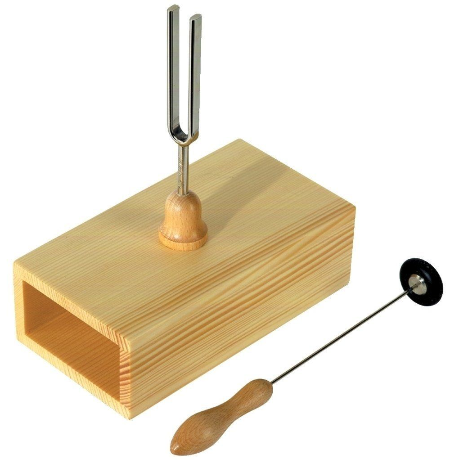
The natural frequency of a typical tuning fork is 440Hz and can be excited using a striker, for example. The wooden body underneath the tuning fork is called the resonance body. If the tuning fork begins to vibrate at its natural frequency, the resonator also begins to vibrate and amplifies the sound. If the tuning fork is only struck once, the sound fades after a short time. The acoustic vibration is damped.
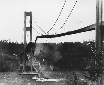
If a system is periodically excited at its natural frequency and is only weakly damped, the amplitude of the oscillation can continue to increase until a resonance catastrophe occurs. In this case, the vibrating system can no longer withstand the vibration amplitude and is destroyed. A popular example is the Tacoma-Narrows Bridge, which collapsed in 1940 due to a resonance catastrophe and can be seen in Figure 3. Prior to this, periodic gusts of wind had caused the bridge to vibrate strongly.
Resonances can occur in any circuit with reactive elements. A simple oscillating system is formed by a capacitance and an inductance. Energy is stored in the electric field when the (ideal) capacitor is charged and converted into magnetic energy via the (ideal) coil when it is discharged. This process is repeated periodically. In the case of resonance, the system is excited at a frequency close to its natural frequency. The simplest real electrical resonant circuits are a series and a parallel resonant circuit, each consisting of a capacitor, an inductor and a resistor. They can be seen in Figure 4. The energy losses at the coil and capacitor are summarized in the ohmic resistance R. Compared to coils, the energy losses at the capacitors are in the range of 0.1 to 1 per thousand, which is why R is always connected in series with L in Figure 4.
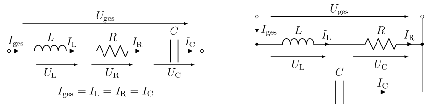
The behavior of the parallel resonant circuit (on the right in Figure 4) is examined in more detail below. The complex impedance Z of the parallel resonant circuit is calculated as follows
$$ Z(f) = \frac{1}{\frac{1}{R + j 2 \pi f L} + j 2 \pi f C} = \frac{R}{\left(1 – (2 \pi f)^2 C L \right)^2 + (2 \pi C R)^2} + j \frac{2 \pi f (C R^2 – L) – (2 \pi f)^3 C L ^2}{\left(1 – (2 \pi f)^2 C L \right)^2 + (2 \pi f C R)^2} $$
and is dependent on the frequency f. If the circuit is operated with the resonant frequency(R→ 0)
$$ f_R = \frac{1}{2 \pi L} \sqrt{\frac{L}{C} – R^2} \approx \frac{1}{2 \pi \sqrt{L C}} $$
the imaginary part of the impedance disappears and the circuit behaves like a high-impedance load towards the terminals. If the series resistance R of the coil is very small, the approximation of the resonant frequency for ideal components from the above formula can be used. If the value of the impedance of the parallel resonant circuit is plotted against the frequency f, it reaches its maximum at resonance. This can be seen in Figure 5.

The resonant circuit exhibits an inductive behavior for f ≪fR and a capacitive low impedance behavior for f ≫fR. Accordingly, the phase of the impedance has a zero crossing at the resonant frequency, as can be observed in Figure 6.

Series and parallel resonant circuits are dual circuits. For this reason, the opposite behavior can be observed for the series resonant circuit at the resonant frequency. The magnitude and phase of the series resonant circuit are shown in Figure 7 and Figure 8. For f ≪fR, the series resonant circuit exhibits capacitive and for f ≫fR inductive high-impedance behavior, while the impedance becomes minimal at the resonant frequency.


The following values were assumed to create the graphs above: L= 100mH, C= 0.92µF and R= 1Ω. The values are typical for an overhead cable with a length of 100 km. The resonance frequency is approx. 500Hz. If the bandwidth of the resonance is to be changed, this can be achieved by using a higher resistance value, for example. In contrast to overhead cables, this is the case with underground cables, which are often used in the medium and low-voltage grid. With a higher resistance, the vibration is damped more and the resonance is less pronounced. At the same time, higher ohmic losses are realized in the resonant circuit. For the following Figures 9 and 10, the resistance was increased to R= 100Ω.


The resonant frequency is not increased in the ideal series resonant circuit by changing the resistance. It can be influenced by varying the inductance or capacitance. In energy transmission systems, for example, this is achieved by using double conductors that reduce the inductance.
In real energy transmission systems, resonances can occur at any frequency due to the interconnection of the large number of operating resources. Depending on the magnitude and phase characteristics, the resonances in an impedance curve can then be divided into parallel and series resonances.
How are impedance, resonances and power quality related?
The interconnected grid consists of a large number of interconnected operating resources. All of this equipment – for example, lines, transformers or consumers – exhibit different behavior depending on the excited frequency. In other words, the electrical energy grid is a huge coupled resonant circuit consisting of capacitive, inductive and resistive elements with several resonant frequencies. If the grid impedance is measured over a longer period of time from any grid connection point (NVP), it will change constantly depending on which loads or feed-ins are being switched on or off. A grid connection point can be modeled by a Thévenin equivalent circuit diagram consisting of an ideal voltage source and an impedance connected in series. For the low and medium voltage range, resistive and inductive components of the grid impedance dominate. For this reason, the grid connection point can be represented as shown in Figure 11.
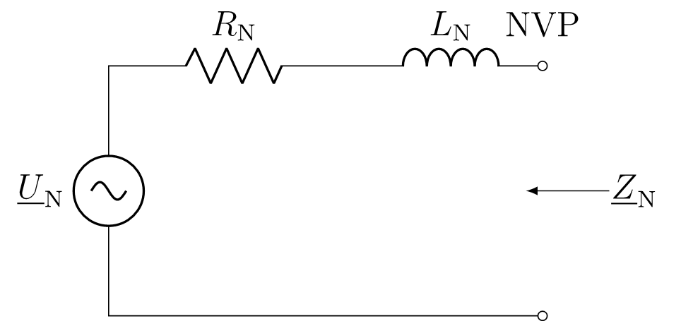
Here \(\underline{U}_N\) denotes the nominal voltage of the grid. If an ohmic resistor with a defined value is connected to the grid connection point, the current and voltage can be measured and the grid impedance calculated from this. The broadband excitation required to measure the spectral grid impedance \(\underline{Z}_N\) is carried out via a randomly generated pulse sequence, after which the resistor is connected to the grid. Figure 12 shows an example of the measured spectral mains impedance on a connector strip with a connected computer power supply from 0 to 150kHz. The magnitude is shown in blue, while the phase is represented by the green curve.

The parallel resonance at approx. 80kHz is clearly recognizable. The magnitude of the mains impedance is maximum at this frequency while the phase has a zero crossing. In this case, the resonance was caused by the capacitive input filter of the computer power supply.
However, it is not only resonances that can be detected by measuring the spectral grid impedance. Grid perturbations can also be identified on the basis of peaks in the measurement curve. Grid perturbations refer to high-frequency currents that are fed back into the power supply grid and thus increase the harmonic content of the grid voltage and current. As explained in the previous section, high-frequency currents are increasing primarily due to the increasing number of power-electronically coupled generators and consumers. If the frequency of the harmonic currents meets series resonances (low impedance), very high currents can flow unhindered and thus damage equipment. Continuous power quality measurements in combination with impedance measurements for resonance detection can detect damage and failures caused by harmonic currents.